Multinomial logit models are a workhorse tool in marketing, economics, political science, etc. One easy and flexible way to estimate these models is in Stan. The reason I like Stan is that it allows you extend beyond the standard multinomial logit model to hierarchical models, dynamic models and all sorts of fun stuff. (If you are interested in hierarchical-Bayes, you should also check out the tutorial that Kevin Van Horn and I wrote.)
However, for beginners, the learning curve can be a bit steep. I set many students to the task of fitting a basic multinomial logit model in Stan. They usually master the Stan syntax get the modeling running pretty quickly, but often the first set of posterior draws and estimates they get from Stan don’t make sense.
Almost always, the problem is that they have misspecified the intercepts in the model. You see, multinomial logit models are a bit quirky in that relative differences in utility between alternatives are identified, but not absolute differences in utility. In practice, this means that if you observe choices from among K alternatives, then you can only estimate K-1 intercept parameters.
The examples in this post illustrate the bad things that happen when you specify K intercept parameters and show several different ways to specify K-1 identified intercept parameters. Along the way, I hope to teach you something about how to test Stan code to see that it recovers the parameters of synthetic data (but see Michael Betancourt’s blog for a much more through treatment) and how to diagnose identification problems.
Before we get started, here are the packages and options I use:
library(rstan)
library(bayesplot)
library(gtools) # rdirchlet
rstan_options(auto_write=TRUE) # writes a compiled Stan program to the disk to avoid recompiling
options(mc.cores = parallel::detectCores()) # uses multiple cores for stan
Data generation for multinomial logit model
The data setup I’ll be working with is typical of many marketing problems where we observe a series of choices from a fixed set of alternatives (often brands of consumer goods) and want to estimate intercepts for each of the alternatives (which we sometimes interpret as “Brand Equity”).
I start every modeling project by writing a function to simulate data from the model. Here is a function for generating synthetic data from the multinomial logit.
generate_mnl_data <- function(N=1000, K=2, J=3, beta=c(1, -2), alpha=c(1,0,-1)){
  if(length(beta) != K) stop ("incorrect number of parameters")
  Y <- rep(NA, N)
  X <- list(NULL)
  for (i in 1:N) {
    X[[i]] <- matrix(rnorm(J*K), ncol=K)
    Y[i] <- sample(x=J, size=1, prob=exp(alpha+X[[i]]%*%beta))
  }
  list(N=N, J=J, K=K, Y=Y, X=X, beta=beta, alpha=alpha)
}
d0 <- generate_mnl_data()
This function creates data where the alternatives for each choice task are stored as a matrix. For instance in d0, there are J=3 alternatives each with K=2 attributes in every choice task. These matrices are stored together in a list of length N for the N choice observations. The attributes for the first observed choice are:
d0$X[[1]]
           [,1]       [,2]
[1,]  1.5523454 -1.3758700
[2,]  0.5406288 -0.4640548
[3,] -0.1771788  1.3438338
We also have a vector Y that indicates which alternative was chosen for each of the N choices. In the first choice, alternative 1 was chosen:
d0$Y[1]
[1] 1Basic multinomial logit model without intercepts
We start by estimating a basic multinomial logit model without intercepts. The Stan code below specifies that model with uniform priors on the parameters.
m1 <-
"data {
  int<lower=2> J; // of alternatives/outcomes
  int<lower=1> N;  // of observations
  int<lower=1> K; // of covariates
  int<lower=0,upper=J> Y[N];
  matrix[J,K] X[N];
}

parameters {
  vector[K] beta;  // attribute effects
}

model {
  for (i in 1:N)
    Y[i] ~ categorical_logit(X[i]*beta);
}"
We can create some synthetic data using generate_mnl_data() and then pass it into the stan() function along with our model code m1 to produce draws from the posterior:
On my machine, this code is fast (<3 sec / 1000 iterations for N=1000) and does not produce any warnings. We can make a traceplot of the draws for beta to see that Stan’s HMC algorithm is performing well:
mcmc_trace(As.mcmc.list(p1, pars="beta"))
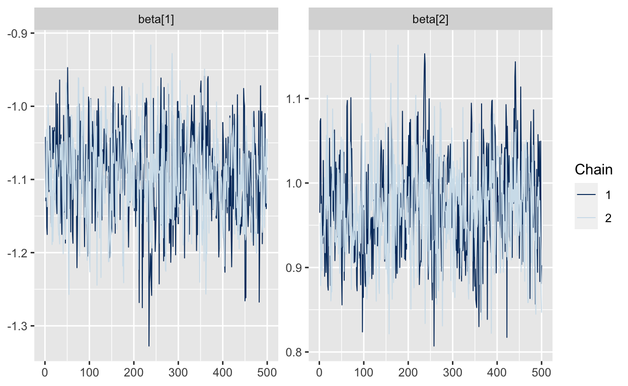
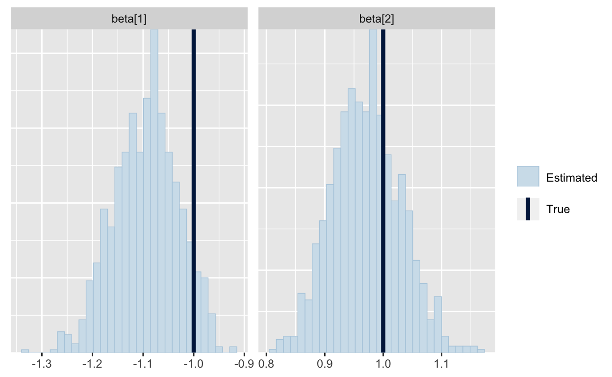
We can also see that the the “true” beta parameters are well within the posterior range, suggesting that the code is working. (There are more through tests we could do, but we’ll skip those for now. (Again, see Betancourt’s blog for more detail.)
mcmc_recover_hist(As.mcmc.list(p1, pars="beta"), true=d1$beta)
The bad way to do MNL with intercepts
The model we estimated above does not include intercepts. In a logit model for data like this, we might want to specify an intercept for each alternative, indicating how much each alternative is preferred. These are sometimes called “alternative specific constants.” I’m going to start by naively specifying a vector alpha, which contains the three intercepts for the three alternatives. Like any other intercepts, I add them to the linear preditor: alpha + X[i]*beta. (If you are having trouble with the matrix algebra, remember alpha is 3 x 1, X is 3 x 2 and beta is 2 x 1. The resulting linear predictor is 3 x 1, i.e. a utility for each alternative.)
m2 <- "
data {
  int<lower=2> J; // of alternatives/outcomes
  int<lower=1> N;  // of observations
  int<lower=1> K; // of covariates
  int<lower=0,upper=J> Y[N];
  matrix[J,K] X[N];
}

parameters {
  vector[J] alpha; // unconstrained intercepts
  vector[K] beta;
}

model {
  for (i in 1:N)
    Y[i] ~ categorical_logit(alpha + X[i]*beta);
}"
Then we can generate data and run the model:
Uh-oh. This looks bad! The code runs very slowly runs slowly (~10 min / 1000 draws for N=1000 on my machine) with lots of warnings from Stan about how the HMC sampler is performing. The traeplots below show that the values of the intercepts in alpha don’t coverge; they just “wander around” to any value. The betas seem to converge, but are mixing poorly. What’s going on here?
mcmc_trace(As.mcmc.list(p2, pars=c("alpha", "beta")))
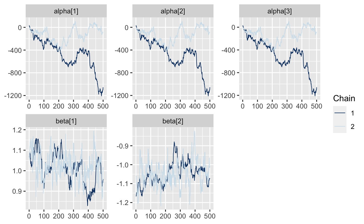
The problem is that the parameters in alpha are not identified. We can add any value to all three intercepts in alpha and the conditional logit likelihood will be the same. And Stan is telling us that by letting the alpha parameters drift all over the place. But we are at the point where the posterior of alpha is so flat that the HMC algorithm starts to perform very slowly.
MNL with prior on intercepts
We are Bayesian, so one way to solve this identification problem is to put informative priors to identify intercepts. Here I specify a fairly tight normal prior for alpha which will keep all three values of alpha fairly close to zero. (Actually, since we didn’t specify a prior in the models above, Stan defaulted to an implicit uniform prior on alpha and beta. This is a really bad prior, but it didn’t matter in the first example because the data identified the beta parameters.)
m3 <- "
data {
  int<lower=2> J; // of alternatives/outcomes
  int<lower=1> N;  // of observations
  int<lower=1> K; // of covariates
  int<lower=0,upper=J> Y[N];
  matrix[J,K] X[N];
}

parameters {
  vector[J] alpha;
  vector[K] beta;
}

model {
  alpha ~ normal(0,1); // prior contrains alpha
  for (i in 1:N)
    Y[i] ~ categorical_logit(alpha + X[i]*beta);
}"
When I run this model, things go much more smoothly.
p3 <- stan(model_code = m3, data=d2, iter=1000, chains=2, seed=19730715)
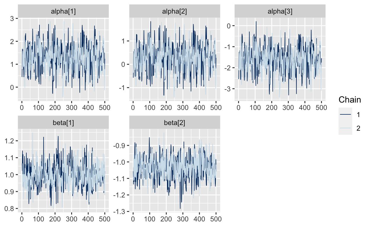
This runs faster (~30s / 1000 iterations) without producting errors and we can see from traceplots that that the values of alpha are now converging and the beta parameters are mixing nicely:
mcmc_trace(As.mcmc.list(p3, pars=c("alpha", "beta")))
And now it looks like the true values we used to generate the data fall within the estimated posteriors.
mcmc_recover_hist(As.mcmc.list(p3, pars=c("alpha", "beta")), true=c(d2$alpha, d2$beta))
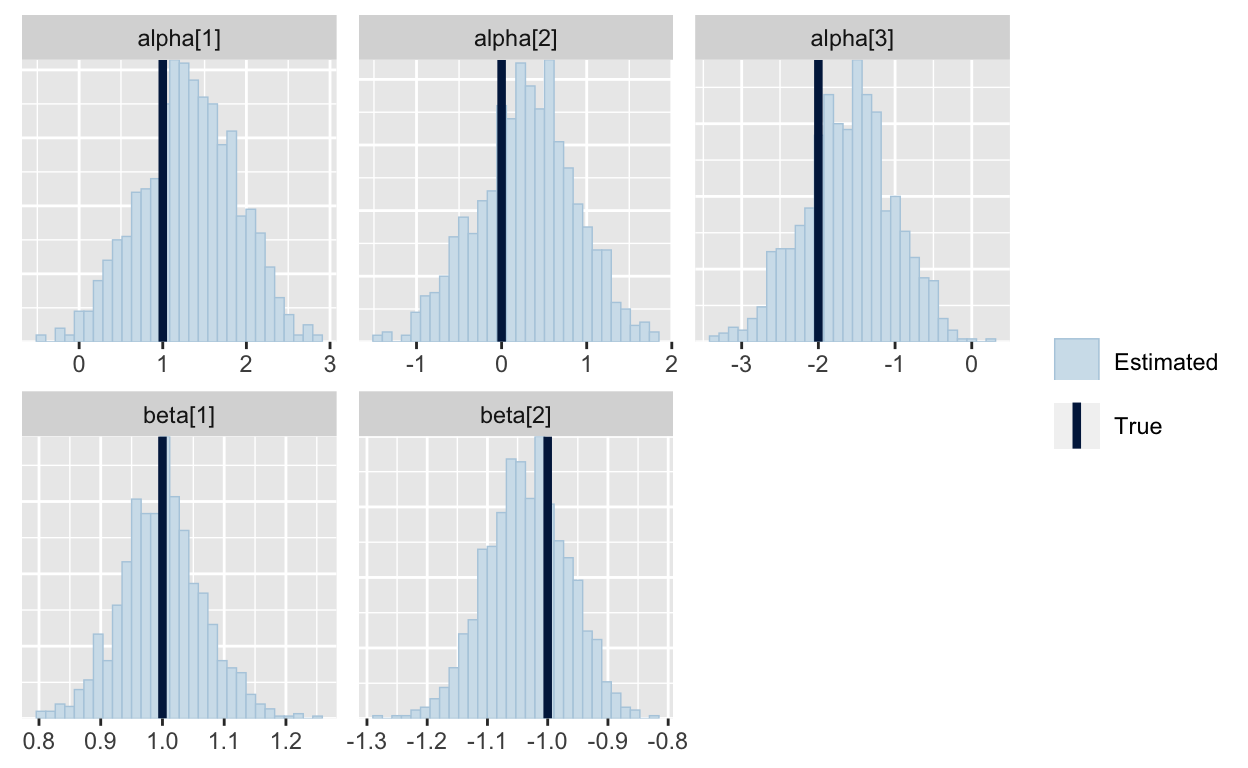
Hurray for priors!
Well, sort-of. This solution works with this data, but if the true value of alpha was 1000, then these priors would be too tight. So, you would have to adjust the priors on alpha depending on your data and that would be a hassle and it generally is better practice to fit models that are fully-identified only by the model and the data.
MNL with fix-one-to-zero constraint
Instead of using priors to constrain the intercepts, a more common identification strategy is to fix one of the intercepts in alpha to zero. One way to accomplish this in Stan is to create a vector of length J-1 which we will call alpha_raw and then appending a zero to it in the transformed parameters block. (Alternatively, you could include J-1 dummy variables for intercepts in X.)
m4 <- "
data {
  int<lower=2> J; // of alternatives/outcomes
  int<lower=1> N;  // of observations
  int<lower=1> K; // of covariates
  int<lower=0,upper=J> Y[N];
  matrix[J,K] X[N];
}

parameters {
  vector[J-1] alpha_raw;
  vector[K] beta;
}

transformed parameters {
  vector[J] alpha;
  alpha = append_row(0, alpha_raw);
}

model {
  for (i in 1:N)
    Y[i] ~ categorical_logit(alpha + X[i]*beta);
}"
This is identified (with just the default uniform priors) and runs quite fast (~7s per 1000 iterations with N=1000).
p4 <- stan(model_code = m4, data=d2, iter=1000, chains=2, seed=19730715)
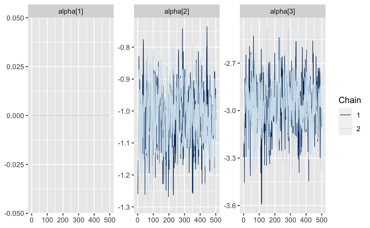
The traceplots now look great even without specifying non-uniform priors: Note that all the values for alpha[1] are zero, because that’s how we defined alpha in the tranformed parameters block.
mcmc_trace(As.mcmc.list(p4, pars=c("alpha")))
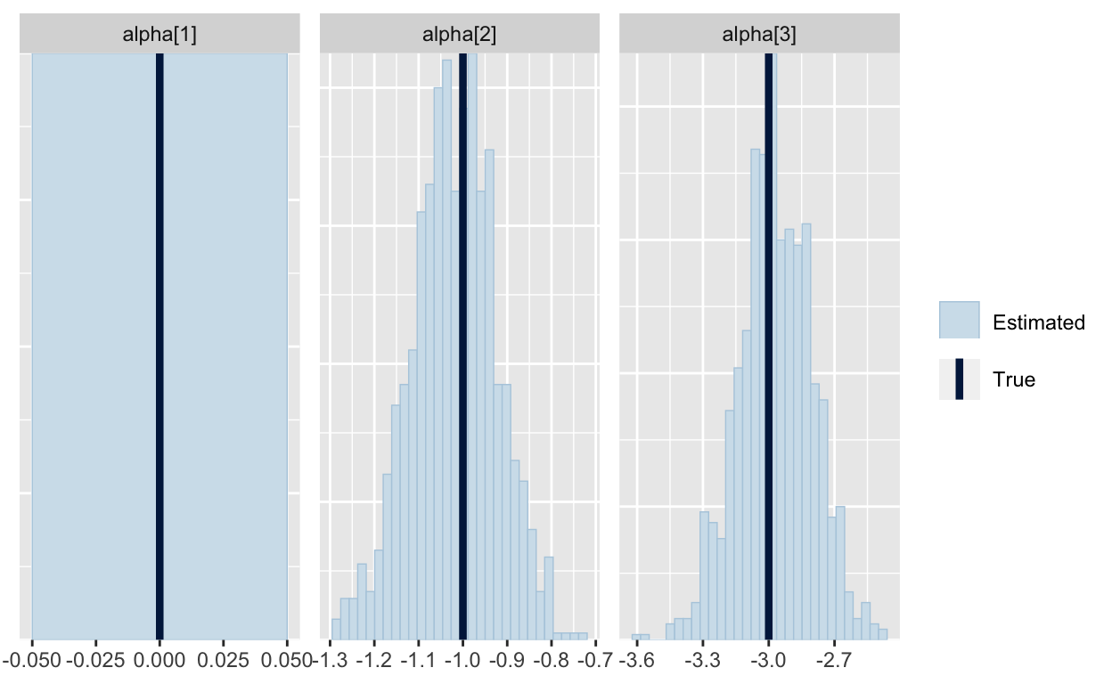
Now, one thing that may be bothering you is that the estimates for alpha are not the values we used to generate the data. The estimates are actually differences between the arbitrarily chosen intercept that was set to zero and the other intercepts. We can compute these differences and then compare them to the posteriors.
shifted_alpha <- d2$alpha - d2$alpha[1]
mcmc_recover_hist(As.mcmc.list(p4, pars="alpha"), true=shifted_alpha)
All looks good and it would be perfectly fine to use this sampler. In fact, this is the specification the mlogit package and in most of the commercial software for the multinomial logit. I see lots of papers in marketing and econ that use this specification.
But it isn’t what I use in my own work. The tricky thing about setting one value of alpha to zero is that it is becomes harder to put priors on alpha_raw. In the example above alpha_raw is defined as the differences in utility. To put priors on alpha_raw, you have to specify your beliefs about the differences in utility each alternative and the base alternative. That can be a hard thing to think about, especially when you are using hierarchical priors to account for heterogeneity in the intercepts across different decision makers. (It is especially bad, if you are trying to compute Bayesian d-optimal designs, as Kevin Van Horn and I once found out the hard way – but that’s beyond the scope of this post.)
MNL with sum-to-zero constraint (but with a very bad Stan implementation)
Instead, I prefer to use a sum-to-zero constraint on alpha, which avoids making one of the alternatives special. The idea behind a sum-to-zero constraint is that we want to constrain sum(alpha) = 1. Here is one very bad way to implement it in Stan. It does recover the true values of the parameters, but because the parameter alpha_raw is unidentified, the HMC sampling is slow and generates lots of warnings.
m5 <- "
data {
  int<lower=2> J; // of alternatives/outcomes
  int<lower=1> N;  // of observations
  int<lower=1> K; // of covariates
  int<lower=0,upper=J> Y[N];
  matrix[J,K] X[N];
}

parameters {
  vector[J] alpha_raw; // unconstrained UPC intercepts
  vector[K] beta;
}

transformed parameters{
  vector[J] alpha;
  alpha = alpha_raw - (1.0/J) * sum(alpha_raw); // sum to zero constraint
}

model {
  // model
  for (i in 1:N)
    Y[i] ~ categorical_logit(alpha + X[i]*beta);
}"
p5 <- stan(model_code = m5, data=d2, iter=1000, chains=2, seed=19730715)
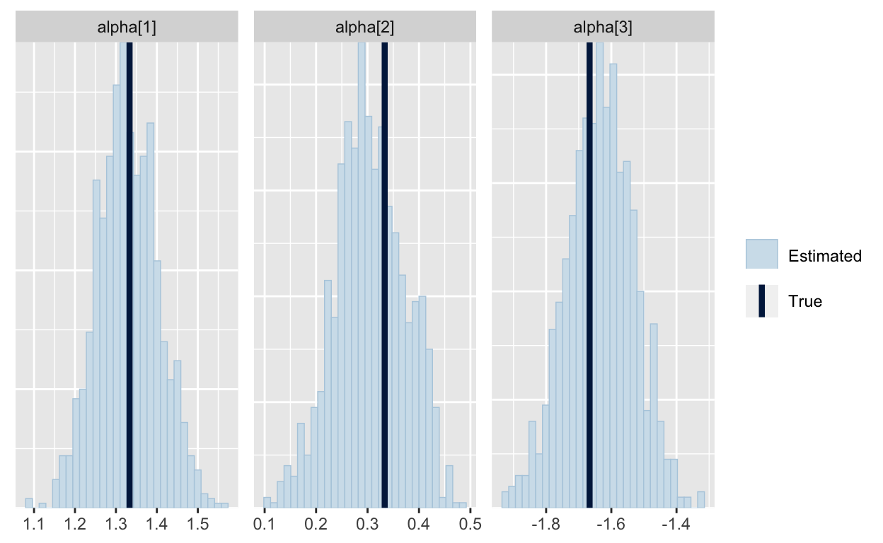
We are getting the true values of alpha back (after shifting them to account for the sum-to-zero constraint):
shifted_alpha = d2$alpha - (1/d2$J)*sum(d2$alpha)
 mcmc_recover_hist(As.mcmc.list(p5, pars="alpha"), true=shifted_alpha)
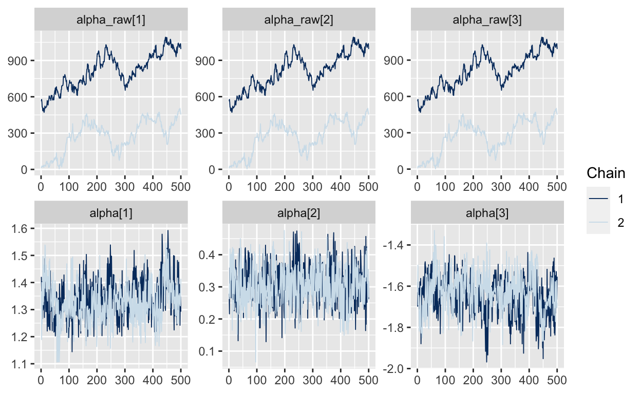
but these traceplots for alpha_raw look awful and it took a long time to get them! (For those of you who have built Gibbs samplers, it actually works very well to sample the unidentified alpha_raw in a Gibbs sampler, but for HMC, not so much.)
mcmc_trace(As.mcmc.list(p5, pars=c("alpha_raw", "alpha")))
MNL with sum-to-zero constraint (better implementation)
Here is a better implementation of the sum-to-zero constraint. Let’s specify alpha_raw as a J-1 vector. By putting this J-1 parameter in the parameters block, we are telling Stan to focus on estimating the J-1 identified parameter in alpha_raw. Then we will create an J vector alpha in the transformed parameters, but instead of putting in 0 for the left-out parameter in alpha, we will use -sum(alpha_raw). This results in an alpha that sums to zero, which we then use to compute the categorical_logit likelihood. This runs fast and smoothly.
m6 <- "
data {
  int<lower=2> J; // of alternatives/outcomes
  int<lower=1> N;  // of observations
  int<lower=1> K; // of covariates
  int<lower=0,upper=J> Y[N];
  matrix[J,K] X[N];
}

parameters {
  vector[J-1] alpha_raw; // unconstrained UPC intercepts
  vector[K] beta;
}

transformed parameters{
  vector[J] alpha;
  alpha = append_row(-sum(alpha_raw), alpha_raw); // sum to zero constraint
}

model {
  for (i in 1:N)
    Y[i] ~ categorical_logit(alpha + X[i]*beta);
}"
p6 <- stan(model_code = m6, data=d2, iter=1000, chains=2, seed=19730715)
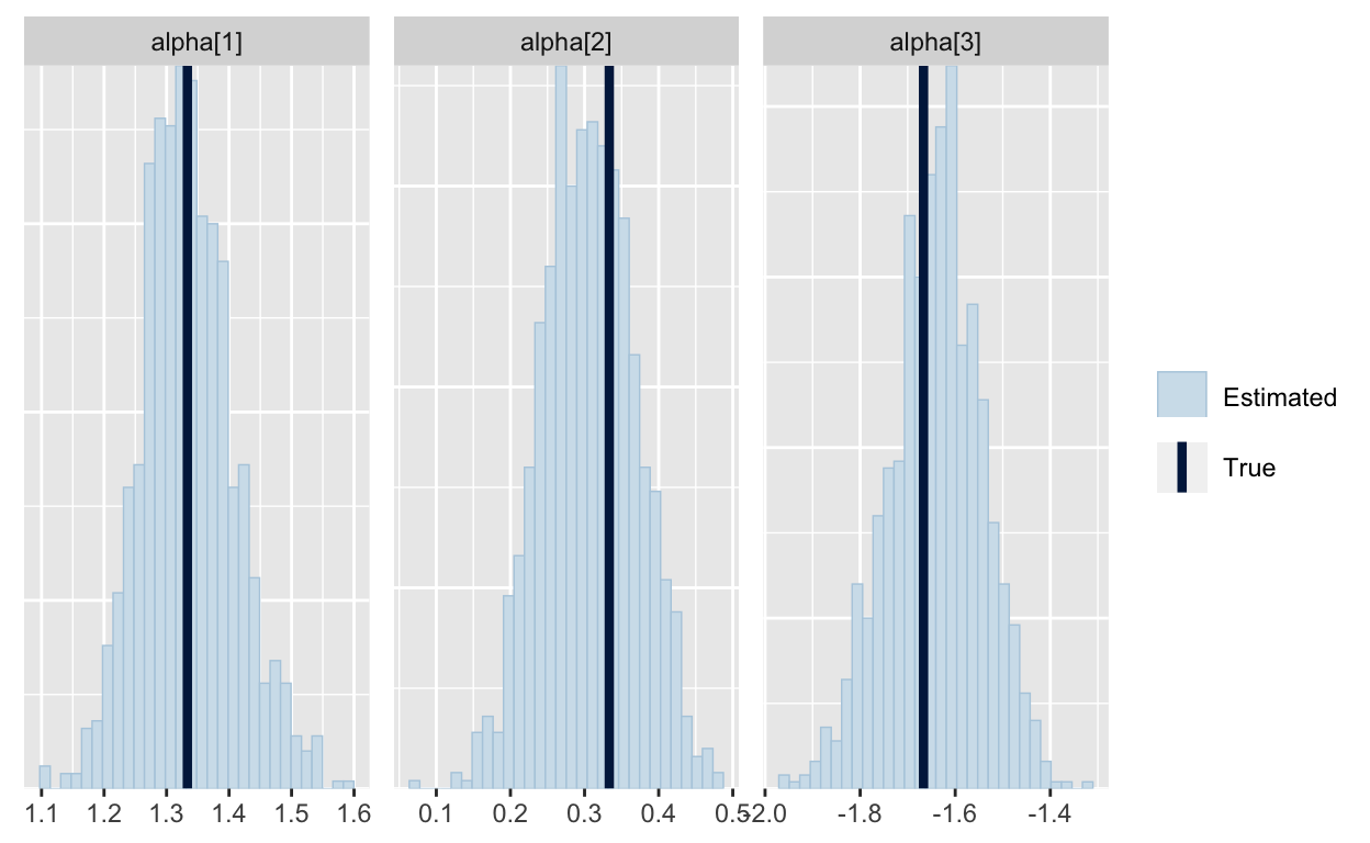
And we can see the true parameters are recovered (after we shift them to account for the sum-to-zero constraint).
shifted_alpha = d2$alpha - (1/d2$J)*sum(d2$alpha)
mcmc_recover_hist(As.mcmc.list(p6, pars="alpha"), true=shifted_alpha)
This specification does not treat the first alternative as special. Instead, the parameters of alpha are the difference in utility between the alternative and the average of all alternatives. (You can see that in how I defined shifted_alpha above.) So, when you specify a prior on the elements of alpha, you can think about how much of a difference you expect to see between any alternative and the average alternative; this works very well in hierarchical models.
So, that’s how to identify intercepts in multinomial logit models. Along the way we learned that:
Before using any estimation procedure on real data, you should run it on synthetic data (simulated from the same model) to make sure it is recovering the parameters correctly. Better yet, run it on many different synthetic data sets. (See Betancourt.)
A slow running Stan sampler with lots of errors is a sign that your model is poorly-specified and may have an indentification issue.
Indentification can be achieved by specifying tighter priors or by applying constraints to the model.